Calibration is the process of adjusting model structure and parameters to try to make model behavior conform to observed behavior, typically time series data measured for some subset of the model variables. Calibration is an important part of building confidence in models and an integral step in the iterative process of identifying, analyzing, and solving problems using dynamic modeling. In our discussion, we will stick to the fairly mechanical definition of calibration supported directly by the software, but it is important to keep in mind that it is a more general concept.
There are four basic steps in calibration: Defining a payoff; specifying parameters to adjust; executing the calibration; evaluating the results.
In order to adjust model parameters to make the model look more like measured data, it is necessary to specify how good a job the model does of matching the data. This is the realm of statistics, and there are a variety of statistical models, and approaches, that can be used to say how well a model matches data. A common approach is least squares, which is derived from statistical models that assume normally distributed error terms. In Stella we call this simply Squared Error. Squared errors give successively higher weight to outliers which, when working with many different data series, tends to make one or two of the series dominate the calibration results. To get around this the alternative error measurement of the absolute value of the error can be used. In Stella we refer to this simply as Absolute Error.
The payoff is computed by comparing model variable values against measured data, or potentially another model variable. The squared or absolute value of this difference is taken and then weighted by a variable specific value and added into the payoff.
See Defining Calibration Payoffs for the mechanics of setting up payoff definitions.
In setting up a comparison you first select the model variable you want to compare, and then the model variable and run you want to compare this two. Most commonly, the value being compared to is data that is brought in via the mechanism of loading data as a run (see Data Manager) or importing time varying data (see Import Data dialog box). In the first case the comparison variable will be the same as the model variable but in a different run, in the second it will be a different variable but in the current run. In both cases, Stella will only use the available data points, not any interpolated values, to make the comparison.
You can also compare to another model variable that is not imported. This might be useful, for example, in calibrating a simplified structure to a more complete model, but we will not go into discussion of such specialized usages.
The payoff is computed by adding up the error measurements across time and across variables. Since different variables will be included, it is necessary to select a weight for each that will make the error measurements, commensurate. This can be done directly based on your understanding of the variables (the units of measure, expected error in computing them and so on), or the software can do it automatically. When done automatically, the software will choose weights so that the value of the payoff is approximately equal to the number of data points. In the case of Squared Errors this gives a payoff that behaves the same as the negative value of the log likelihood in terms of its response to parameter changes. In the case of the Absolute Errors there is no strong statistical basis, but the reported payoff will still have a well-defined value range.
It is important to note, that assumptions giving a payoff equal to the number of data points are based on the expectation that the average values of the variable and data are approximately equal. If the variable is always lower (or higher) than the data the payoff will be larger than the number of data points.
Stella allows you to specify a tolerance when computing the error for each variable. These are typically 0, so that the error increases continuously as the model computation moves away from the data. There are some cases, however, for which a variable being close to the data is the same as it matching the data exactly. Setting a nonzero tolerance will allow that to happen. For any values within 90% of that tolerance it will be the same as if the value exactly matched the data. Between 90% and 100% of the tolerance the value adjusts smoothly to the value without a tolerance, thus ensuring continuity which is helpful for the solution process.
The selection of parameters to adjust needs to be based on your understanding of the model structure. Mechanically, it is identical to the set-up of parameters for optimization (see Optimization Specs).
You can make use of any of the available options for controlling an optimization (see Optimization Specs). Once those are set up you simply click on Run in that panel, or O-Run on the toolbar. The calibration will proceed and the result will be put into the simulation log.
Mechanically, the purpose of the calibration is to make the model behavior look like the data. Conceptually, the purpose of the calibration is to make a judgment about model quality based on the mismatch between the model behavior and the data. Such a judgment can only be made after work has been done to minimize that mismatch. Put another way, we can use data as one basis for rejecting our hypothesis that the model we built is helping us to understand a problem. Put in a more nuanced way, the mismatch can help us see shortcomings in our model. In every case, however, we need to get the model to the point where the mismatch is as small as it can be given the model structure.
If you have been able to independently compute payoff weight, the payoff value itself can be used as one measure of model quality. If you are automatically computing weights, however, you will need to look at the individual payoff components to understaffed how well things line up and what kind of issues might be causing mismatches. This is typically done with comparative graphs and tables, and involves the same type of analysis done more generally in understanding model behavior.
Confidence bounds are an indication of how tightly you have been able to estimate the parameter values. If you select the option to compute confidence bounds in the Optimization Specs panel the software will move away from the optimal value for each parameter until the specified tolerance is reached. For payoffs that use a sum of squares, this tolerance is determined by specifying a percent (95% by default) and finding the change that result in a deviation from that. Put another way, it will be 95% certain that the parameters fall within the range determined. For other types of payoff you will need to determine the amount the payoff should be changed to understand the meaning of the range found.
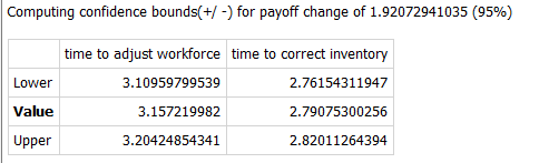
In the above example it says that there is 95% certainty that the value of the time to adjust workforce lies between 3.1 and 3.2 and that the value of time to correct inventory lies between 2.76 and 2.82. This percent corresponds to a change in payoff of 1.9. That is, if the payoff reported was 1000 for a value of time to adjust workforce of 3.15, then setting time to adjust workforce to 3.1, or 3.2 would give a payoff of 1002.
Note If the Lower or upper value is reported as * it means that the corresponding bound could not be found. This can happen when changes in the parameter do not make the payoff consistently worse, or when the value found is very close to the minimum or maximum value allowed. A * for the value may occur when a parameter is at a minimum or maximum and the payoff could be improved by exceeding the bound.
The above example assumed squared errors and automatically computed weights, so the percent bounds can be used and the appropriate range calculated. But even when the meaning of the change in payoff is difficult to interpret, the relative ranges can be very helpful in understanding which parameters are important to keep at a value near that found by the calibration process. For example, you might be calibrating to determine the best values for the perception delay for product and service quality. In doing so you might find that product quality perception has a delay of 8 months with a range between 3 and 20, while service quality has a delay of 3 months with a range of 2 to 4 months. In this case we are learning much less from the calibration process about perceived product quality than we are about perceived service quality.